Diversions in Mathematics 3a: The Cauchy-Schwarz inequality (part 1)

Preface

After a long time, I have decided to resurrect the mathematics part of this blog! I started Diversions in Mathematics as a way for me to try to explain mathematics to the general public. This continues to be the main goal of this series of blogposts — for a more detailed introduction, please read the introductory remarks. I wrote two posts in this series, but then abruptly stopped. Part of the reason was that my studies got in the way, but I was also unsure exactly what material to present, and how to present it. I wrote down some of my thoughts on this matter in a previous update post.

One of the main issues as a writer is to consider the readers’ background in mathematics. For posts targeting the general public (like the previous two Diversions), I have tried to assume as little as possible while maintaining the discussion at an intelligent level, i.e. without “dumbing down” anything) However, this already assumes familiarity with many mathematical concepts taught in high school, or at least, some level of maturity in regard to abstract reasoning. Consequently I have decided to relaunch Diversions in Mathematics with high school mathematics as a foundation.

In this blogpost, I will introduce the Cauchy-Schwarz inequality, one of the most fundamental results in mathematical analysis, with the aim of connecting various topics that are typically studied in the Year 12 HSC maths curriculum in NSW. The main article is below.

Equations vs. Inequalities

Much of the high school maths curriculum, for better or worse, is devoted to methods of solving equations. Do the following exercises ring a bell?

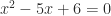
Homework Exercise (due on Monday): For each of the following equations, find all solutions $x$ in the real numbers.

$2x - 5 = 11$
$x^2 - 5x + 6 = 0$
$x^2 + 1 = 0$
$e^{-4x} = \frac{1}{2}$
$\sin(\pi x) = \frac{\sqrt{3}}{2}$

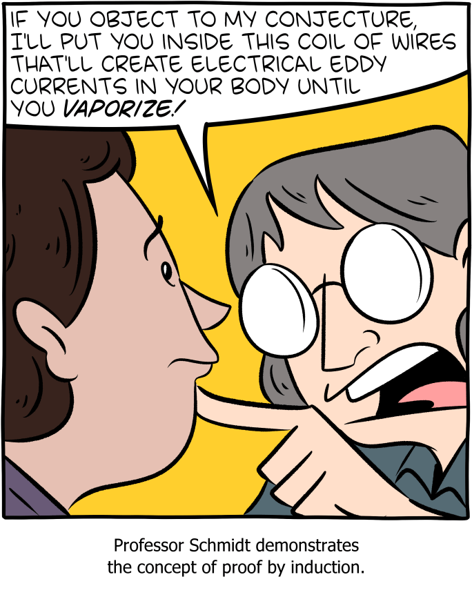
I hope this doesn’t induce traumatic memories. As an unfortunate consequence, I suspect that many people have the impression that maths is just about solving equations. This is far from the truth! I am rather fond of this cartoon from Ben Orlin:

The cartoon comes from this article, which I recommend to read.

Of course, learning to solve equations is extremely important and useful. However, the key point I want to raise is that tackling inequalities often requires a set of tools that is quite different from those used to solve equations. A solution to an algebraic equation, as in my hypothetical homework exercise above, is simply a number. This is a quantitative statement: we are affirming that when the variable $x$ is equal to a certain number, it satisfies the desired formula. On the other hand, the study of inequalities gives the opportunity to consider qualitative statements. For example, if $f(x)$ is a given function, then the statement

$|f(x)| \le 1$ for all $x \in \mathbb{R}$

says that the absolute value of the output $f(x)$ is bounded above by 1, for real number input $x$ . An equivalent statement is given by

$-1 \le f(x) \le 1$ for all $x \in \mathbb{R}$

It is conceivable that we don’t know the value of $f(x)$ for some input, or even for many inputs $x$ . For example, $f(x)$ could be the solution to a differential equation that is extremely difficult or impossible to solve by hand, and hence we can only estimate the values. Depending on the situation, we may not even care to know the precise values of the function. We could fill many blogposts with discussions on the utility of qualitative information in many aspects of science and humanities. Instead, I want to focus on just one famous inequality in this blogpost. Before we see its proper form, let’s discuss positivity.

Positivity

Given any expression involving an inequality sign $\le, \ge, <, >$ , we can easily transform it into a statement about positivity: the fundamental principle is that if $A$ and $B$ are quantities such that $A \ge B$ , then this is equivalent to the statement that $A-B \ge 0$ , i.e. $A-B$ is positive. [Before we continue, a quick note on terminology. Our convention differs slightly from other texts, where positive means $> 0$ . However, I prefer to avoid double negatives such as “non-negative”. Hence, if $x > 0$ , we will say that “ $x$ is strictly positive” to emphasise the difference from $x \ge 0$ ].

The basis of many inequalities is the following fact:

$x^2 \ge 0$

(for all real numbers $x$ )

Since this is true for all real numbers, we can substitute any other expression for a real number in place of $x$ to obtain many other inequalities. This is a common algebraic trick that ought to be familiar to many students.

As a simple but important example, consider substituting $x-y$ in place of $x$ . Then we can expand out the brackets to obtain $(x-y)^2 \ge 0 \implies x^2 - 2xy + y^2 \ge 0$ , which implies the following classic inequality:

$2xy \le x^2 + y^2 \qquad (\star)$

If $x, y$ are positive numbers, we can replace $x, y$ by their square roots $\sqrt{x}, \sqrt{y}$ in the above inequality, rearrange a little, and obtain

$\sqrt{xy} \le \frac{x+y}{2}$

This is a special case of another famous result, namely the arithmetic-geometric mean inequality (often abbreviated to AGM inequality). Now we are ready to introduce the Cauchy-Schwarz inequality in its simplest form.

Theorem 3.1 (Cauchy-Schwarz inequality)
Let $n \ge 1$ be an integer. Given any two sets of real numbers $\{ x_1, x_2, \ldots, x_n \}$ and $\{ y_1, y_2, \ldots, y_n \}$ , the following inequality holds:

$\displaystyle\sum_{k=1}^n x_k y_k \le \left( \displaystyle\sum_{k=1}^n x_k^2 \right)^{1/2} \left( \displaystyle\sum_{k=1}^n y_k^2 \right)^{1/2}$

This is definitely an unwieldy statement — we will see a dramatic improvement towards the end of this blogpost! We will prove this result by induction (another important HSC topic). However, it is worth examining some simple cases first.

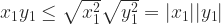
In this case where $n = 1$ , there is almost nothing to prove. The summations reduce to single terms: we have $x_1 y_1$ on the left hand side and $(x_1^2)^{1/2} (y_1^2)^{1/2} = \sqrt{x_1^2} \sqrt{y_1^2}$ on the right. However, recall that if $a$ is any real number, then

$\sqrt{a^2} = |a|$

So the right hand side of the Cauchy-Schwarz inequality is equal to $|x_1||y_1|$ , and we can clearly see that this is larger than or equal to $x_1 y_1$ .

For $n=2$ , the Cauchy-Schwarz inequality reads

$x_1 y_1 + x_2 y_2 \le (x_1^2 + x_2^2)^{1/2} (y_1^2 + y_2^2)^{1/2}$

Suddenly, things are not so obvious! How could we demonstrate the truth of this inequality? The presence of squares and the way that the terms are paired up on the left hand side suggests that we use our starred inequality $(\star)$ from earlier. Then we obtain

$x_1 y_1 + x_2 y_2 \le \frac{1}{2}(x_1^2 + y_1^2) + \frac{1}{2}(x_2^2 + y_2^2) = \frac{1}{2}(x_1^2 + x_2^2) + \frac{1}{2}(y_1^2 + y_2^2)$

Unfortunately, this is not quite right: the right hand side is a bit too large. Indeed, upon a moment’s reflection, perhaps you spot the connection to the AGM inequality $\sqrt{ab} \le \frac{1}{2}(a+b)$ . By setting $a = x_1^2 + x_2^2$ and $b = y_1^2 + y_2^2$ , we deduce

$(x_1^2 + x_2^2)^{1/2} (y_1^2 + y_2^2)^{1/2} \le \frac{1}{2}(x_1^2 + x_2^2) + \frac{1}{2}(y_1^2 + y_2^2)$

Clearly we need to look elsewhere… but we need not go too far. Recall that the simple AGM inequality above was a consequence of $x^2 \ge 0$ followed by various clever substitutions. Could we not deduce the $n=2$ case of the Cauchy-Schwarz inequality by considering the positivity of a certain quantity?

As an initial investigation, let us square both sides of the Cauchy-Schwarz inequality and expand out the brackets:

$(x_1 y_1 + x_2 y_2)^2 \le (x_1^2 + x_2^2)(y_1^2 + y_2^2) \qquad (1a)$

$x_1^2 y_1^2 + x_2^2 y_2^2 + 2x_1 y_1 x_2 y_2 \le x_1^2 y_1^2 + x_1^2 y_2^2 + x_2^2 y_1^2 + x_2^2 y_2^2 \qquad (1b)$

At first glance, this appears to have made things worse, but fortunately, many terms cancel out. We find that the above inequality is equivalent to

$2x_1 y_1 x_2 y_2 \le x_1^2 y_2^2 + x_2^2 y_1^2 \qquad (2a)$

At this point, it is hopefully clear that lurking in the background is the positive quantity

$0 \le (x_1 y_2 - x_2 y_1)^2 = x_1^2 y_2^2 + x_2^2 y_1^2 - 2x_1 y_1 x_2 y_2 \qquad (2b)$

We can now prove the Cauchy-Schwarz inequality in the case where $n=2$ . Starting from inequality (2b), this immediately implies (2a). Adding $x_1^2 y_1^2 + x_2^2 y_2^2$ to both sides of (2a) yields (1b), which can be factorised to produce (1a). Finally, since both sides of (1a) are positive, we may take the square root of both sides, and using the fact that any number is always smaller than its absolute value, we conclude

$x_1 y_1 + x_2 y_2 \le (x_1^2 + x_2^2)^{1/2} (y_1^2 + y_2^2)^{1/2}$

which is the desired result. Observe that we have discovered the steps in the backwards order! This can happen when proving inequalities — very often, a lot of investigation “around” the problem is required before the solution strategy becomes clear.

Inductive proof of Cauchy-Schwarz

Source: https://www.smbc-comics.com/comic/proof

It is about time we tackle the general case. We will proceed by mathematical induction, which is a staple of the HSC examinations (and does not involve electromagnetism). As it turns out, the discussion above has given us all the tools needed to complete the proof!

Base case: $n=1$

In this case, the Cauchy-Schwarz inequality reduces to a statement about real numbers and their absolute values:

$x_1 y_1 \le \sqrt{x_1^2} \sqrt{y_1^2} = |x_1||y_1|$

and we have verified the truth of this statement in the previous section.

Induction step

Now assume that the Cauchy-Schwarz inequality holds for some integer $n \ge 1$ . We will show that it holds for $n+1$ ; that is, we will prove

$\displaystyle\sum_{k=1}^{n+1} x_k y_k \le \left( \displaystyle\sum_{k=1}^{n+1} x_k^2 \right)^{1/2} \left( \displaystyle\sum_{k=1}^{n+1} y_k^2 \right)^{1/2}$

Since we have assumed the result to be true for $n$ terms, it follows that

$\displaystyle\sum_{k=1}^{n+1} x_k y_k \le \left( \displaystyle\sum_{k=1}^{n} x_k^2 \right)^{1/2} \left( \displaystyle\sum_{k=1}^{n} y_k^2 \right)^{1/2} + x_{n+1} y_{n+1}$

At this point, you should be wondering, how can we get the $x_{n+1} y_{n+1}$ to appear inside the square roots? This seems like a very messy operation. However, upon further reflection, you would probably stumble across the idea of using the $n=2$ case of the Cauchy-Schwarz inequality, which we already proved in the previous section! Notice that the right hand side of the result directly above is of the form $a_1 b_1 + a_2 b_2$ , where $a_2 = x_{n+1}, b_2 = y_{n+1}$ and $a_1, b_1$ are the somewhat unwieldy square roots of sums. We know already that

$a_1 b_1 + a_2 b_2 \le \sqrt{a_1^2 + a_2^2} \sqrt{b_1^2 + b_2^2}$

and consequently

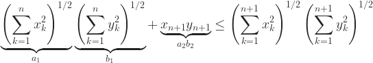
$\underbrace{\left( \displaystyle\sum_{k=1}^{n} x_k^2 \right)^{1/2}}_{a_1} \underbrace{\left( \displaystyle\sum_{k=1}^{n} y_k^2 \right)^{1/2}}_{b_1} +\underbrace{ x_{n+1} y_{n+1}}_{a_2b_2} \le \left( \displaystyle\sum_{k=1}^{n+1} x_k^2 \right)^{1/2} \left( \displaystyle\sum_{k=1}^{n+1} y_k^2 \right)^{1/2}$

This completes the inductive step, and hence proves the Cauchy-Schwarz inequality.

An invitation to a geometric proof

The proof of the Cauchy-Schwarz inequality we have just developed is purely algebraic: as a setup, we used nothing more than a few elementary inequalities, and the conclusion was achieved using the power of inductive reasoning. The x’s and y’s appearing in the inequality can be taken as arbitrary real numbers. However, as I remarked above already, the square root of the sum of squares that appears on the right hand side of the Cauchy-Schwarz inequality is rather unwieldy algebraic expression. Surely, you suspect, there must be something deeper. That expression must have a neater interpretation?

If you suspected this, then you would be absolutely right: the Cauchy-Schwarz inequality is most useful in the context of vectors.

Remark 3.2. The study of vectors has been introduced to the Extension 2 mathematics syllabus in NSW only this year (2020), although it has been in the mathematics syllabus in the Victoria and South Australia examinations for some time already.

Vectors are the foundational tool for mathematics in higher dimensions, and vector spaces are the natural setting for many problems throughout mathematics and hence in all areas of science and engineering. Although the concept of a vector space in general is quite abstract, there is a particular example that is familiar to everyone: the 3-dimensional space we live in. Every point in 3-dimensional space can be described by a set of 3 real numbers — its coordinates — denoted by $(x_1, x_2, x_3)$ , where $(0, 0, 0)$ is an arbitrarily chosen reference point called the origin. In a similar way, mathematicians have no difficulty thinking about points in $n$ -dimensional space, which are of course described by a set of $n$ coordinates, $(x_1, x_2, \ldots, x_n)$ .

In this setting, a vector can be represented as an arrow connecting two points in the space. A vector that is drawn from the origin is called a position vector, since it specifies uniquely the position of some point, say $P$ . Then we can label the vector with the same coordinates as we used for the point $P$ . In the picture below, we have a position vector $\mathbf{u}$ in 2D space (the plane) corresponding to the point $P$ with coordinates $(x_1, x_2)$ . The vector is often written with square brackets $\mathbf{u} = [x_1, x_2]$ to distinguish it from the point $P$ (although this is not universally enforced).

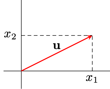
One of the fundamental properties of a vector is its length, or magnitude or norm (the last term is used in more abstract situations). We denote the length of a vector $\mathbf{u}$ using the symbol $\| \mathbf{u} \|$ . For position vectors in the plane, it is easy to see that the length can be calculated using Pythagoras’ theorem. If $\mathbf{u} = [x_1, x_2]$ , then

$\| \mathbf{u} \| = \sqrt{x_1^2 + x_2^2}$

The generalisation to an arbitrary number $n$ of dimensions is quite natural:

$\|\mathbf{u}\| = \left( \displaystyle\sum_{k=1}^n x_k^2 \right)^{1/2}$

Thus, given two vectors $\mathbf{u} = [x_1, \ldots, x_n]$ and $\mathbf{v} = [y_1, \ldots, y_n]$ , the right hand side of the Cauchy-Schwarz inequality is simply $\|\mathbf{u}\| \|\mathbf{v}\|$ , the product of the lengths of $\mathbf{u}$ and $\mathbf{v}$ .

Naturally, you may wonder if we can interpret the left hand side $\sum_{k=1}^n x_k y_k$ in terms of vectors. Indeed, it does appear that there is some kind of “product” operation going on: notice that the left hand side is obtained by taking the product of each pair of coordinates $x_k y_k, k=1, \ldots, n$ , and then summing up everything. As we will see in the next blogpost, such an operation is called a dot product, which is a special case of the very general concept of an inner product on a vector space. The Cauchy-Schwarz inequality demonstrates its full power when generalised to a statement about inner products. In this regard, the inequality has a nice geometric interpretation, and moreover can be derived as a consequence of an optimisation problem. We will discuss these things in the next blogpost!

For the curious reader, I have written a set of notes on the essential vector concepts taught in the HSC syllabus.

One thought on “Diversions in Mathematics 3a: The Cauchy-Schwarz inequality (part 1)”

Pingback: Diversions in Mathematics 3b: The Cauchy-Schwarz inequality (part 2) – Jonathan Mui

Preface

Equations vs. Inequalities

Positivity

Inductive proof of Cauchy-Schwarz

An invitation to a geometric proof

Share this:

Like this:

Related

One thought on “Diversions in Mathematics 3a: The Cauchy-Schwarz inequality (part 1)”

Leave a Reply Cancel reply