Diversions in Mathematics 3b: The Cauchy-Schwarz inequality (part 2)

In the previous post, we introduced the Cauchy-Schwarz inequality purely as a statement about real numbers:

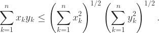
$\displaystyle \sum_{k=1}^n x_k y_k \le \left( \displaystyle \sum_{k=1}^n x_k^2 \right)^{1/2} \left( \displaystyle \sum_{k=1}^n y_k^2 \right)^{1/2}.$

We proved this inequality using mathematical induction. However, one could argue that the method did not yield much insight. As our proof was entirely algebraic, it is not easy to see why the sums that appear in the inequality are reasonable quantities to consider, and there is no hint as to how they could arise naturally in mathematical problems. Therefore, in this post, we will look at the Cauchy-Schwarz inequality from a geometric perspective, which reveals a much richer structure. Moreover, we will see how the inequality arises naturally from a basic optimisation problem.

Note: I continue with the convention from the previous post that a quantity $x$ is called positive if $x \ge 0$ . We say that $x$ is strictly positive if $x > 0$ .

The dot product

Mathematics is all about discovering patterns and relationships between objects (they can be abstract mathematical objects or indeed real-life objects!). Given two vectors, it is quite natural to ask: how can we describe the relationship between them? Can we quantify what it means for a pair of vectors to be “close” to each other? Since we often think of vectors as arrows in space that encode a direction, it makes sense intuitively to consider “closeness” of two vectors as a measure of “alignment” between their respective directions. Here are some pictures to illustrate what I mean:

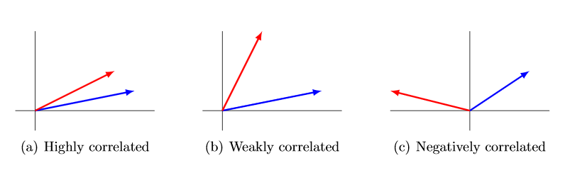
We are therefore looking for some operation that will take two vectors as inputs, and outputs a measure of correlation. If the vectors have unit length, then this operation should also return something that is directly connected to the angle between the vectors. It turns out that the most sensible definition for such an operation is the dot product, defined by:

$\mathbf{u} \cdot \mathbf{v} = \| \mathbf{u} \| \| \mathbf{v} \| \cos \theta$

where $\theta$ is the angle between the two vectors. You may wish to consult Section 3 in my notes on the dot product for a detailed discussion. Notice the dot between the two vectors $\mathbf{u}$ and $\mathbf{v}$ — we do not write $\mathbf{u}\mathbf{v}$ (so it is not a “multiplication”). More importantly, observe that the dot product between two vectors produces a scalar quantity (a real number, not another vector!). This makes sense — after all, our aim was to measure correlation between vectors, and a vector quantity doesn’t seem like a reasonable solution for this purpose.

If we are given the vectors in terms of their coordinates, say $\mathbf{u} = [x_1, \ldots, x_n]$ and $\mathbf{v} = [y_1, \ldots, y_n]$ , then one can derive the formula

$\mathbf{u} \cdot \mathbf{v} = \displaystyle\sum_{k=1}^n x_k y_k$

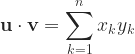
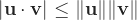
with a bit of trigonometry. To see the details, I refer you again to my notes, where the calculation is done for 3-dimensional vectors, since the notes were designed for HSC students (although the method I used will work in any number of dimensions). Thus the dot product is exactly what appears on the left hand side of the Cauchy-Schwarz inequality! It was already mentioned in the previous post that the right hand side is equal to $\| \mathbf{u} \| \| \mathbf{v} \|$ , the product of the lengths of the vectors. Consequently we can restate the Cauchy-Schwarz inequality in an elegant, compact manner:

Theorem 3.2 (Cauchy-Schwarz inequality)
Let $\mathbf{u} = [x_1, \ldots, x_n]$ and $\mathbf{v} = [y_1, \ldots, y_n]$ be any two vectors. Then the following inequality holds:

$|\mathbf{u} \cdot \mathbf{v}| \le \| \mathbf{u} \| \| \mathbf{v} \|$

Equality holds if and only if $\mathbf{u}, \mathbf{v}$ are linearly dependent, i.e. there exists a scalar $\lambda \in \mathbb{R}$ such that $\mathbf{u} = \lambda \mathbf{v}$ .

Schwarz’s proof

I believe the following proof is due to Hermann Schwarz himself (although I haven’t actually researched this, so I’ll flag this line with [citation needed]). The proof is so slick it almost feels like cheating!

Proof.

Define the function

$p(t) = \| \mathbf{u} + t\mathbf{v} \|^2 \qquad (t \in \mathbb{R})$

Using the fact that $\| \mathbf{x} \|^2 = \mathbf{x} \cdot \mathbf{x}$ for all vectors, we can expand the definition to discover that $p(t)$ is actually a quadratic function:

$\| \mathbf{u} + t\mathbf{v} \|^2 = (\mathbf{u} + t\mathbf{v}) \cdot ( \mathbf{u} + t\mathbf{v}) = \| \mathbf{u} \|^2 + 2t ( \mathbf{u} \cdot \mathbf{v}) + t^2 \| \mathbf{v}\|^2$

(You are encouraged to fill in the details). However, the squared length of any vector is always positive, so that $p(t) \ge 0$ for all $t \in \mathbb{R}$ . It follows that the quadratic $p(t)$ can have at most one real root. Recalling what we learned in high school about quadratic equations, this means that the discriminant of $p(t)$ must be negative. Precisely, we have the following necessary condition:

$[2(\mathbf{u} \cdot \mathbf{v})]^2 - 4 \| \mathbf{v} \|^2 \| \mathbf{u} \|^2 \le 0$

Therefore $4(\mathbf{u} \cdot \mathbf{v})^2 \le 4 \| \mathbf{u} \|^2 \| \mathbf{v} \|^2$ . After cancelling the factor of 4, notice that we can take the square root on both sides, since all quantities involved are positive. Hence we obtain the result $| \mathbf{u} \cdot \mathbf{v}| \le \| \mathbf{u} \| \| \mathbf{v} \|$ . $\Box$

Exercises / Discussion for students

Fill in the details in the proof above, making sure to use the properties of the dot product carefully (e.g. see Section 2 in my notes).
Determine the conditions for equality to hold in the Cauchy-Schwarz inequality. Here’s one way to do it: notice that the argument above shows that equality holds if and only if $p(t) = 0$ . It is also useful to approach this geometrically: since the dot product is supposed to measure correlation between vectors, the condition $|\mathbf{u} \cdot \mathbf{v}| = \| \mathbf{u} \| \| \mathbf{v} \|$ would mean that the vectors are “maximally” correlated. Give a geometric description of this situation.
Given two non-zero vectors $\mathbf{u}, \mathbf{v}$ , the projection of $\mathbf{v}$ onto $\mathbf{u}$ is given by the formula $\text{proj}_{\mathbf{u}} \mathbf{v} = \displaystyle\frac{ \mathbf{u} \cdot \mathbf{v} }{\| \mathbf{u} \|^2} \mathbf{u}$ (see the picture below). Calculate the length of the orthogonal complement $\mathbf{w} = \mathbf{v} - \text{proj}_{\mathbf{u}} \mathbf{v}$ and hence produce a short geometric proof of the Cauchy-Schwarz inequality.

In the next section, we will give yet another proof of the Cauchy-Schwarz inequality that highlights some different techniques.

Cauchy-Schwarz via optimisation

The epsilon trick

You may recall previously that we tried to derive the Cauchy-Schwarz inequality starting with the elementary AGM inequality $ab \le \frac{1}{2} a^2 + \frac{1}{2} b^2$ for all real numbers $a, b$ . This did not directly yield the result, but there is a sneaky trick that we can employ. Observe that the left hand side $ab$ is unchanged if we rescale $a \mapsto \epsilon a$ and $b \mapsto b/\epsilon$ , where the Greek letter epsilon $\epsilon$ denotes an arbitrary, strictly positive number. In this way, we get some extra information “for free” by applying the AGM inequality to these rescaled quantities:

$ab = (\epsilon a) \left( \displaystyle\frac{b}{\epsilon} \right) \le \displaystyle\frac{\epsilon^2}{2} a^2 + \displaystyle\frac{1}{2 \epsilon^2} b^2.$

This epsilon trick is a humble but very useful tool in mathematical analysis! Notice that it has created a certain asymmetry in the inequality. On the left hand side, we have a fixed value $ab$ , but the right hand side now has a free parameter $\epsilon^2$ . We may as well write $\epsilon^2 = t$ to simplify things.

$ab \le \displaystyle\frac{t}{2} a^2 + \displaystyle\frac{1}{2t} b^2$

Making use of the free parameter, we can try to optimise the right hand side, i.e. we seek a value of $t > 0$ that will make the quantity on the right hand side as small as possible. We have a simple calculus exercise.

Exercise for students

Let $a, b > 0$ be given. Prove that the function

$f(t) = \displaystyle\frac{a^2}{2} t + \displaystyle\frac{b^2}{2t}$

defined for all $t > 0$ , achieves its minimum value $ab$ at $t = \displaystyle\frac{b}{a}$ .

Of course, the result of the exercise should not be surprising at all, given what we know about the AGM inequality. However, when used in the context of vectors, the result is more interesting. We show how the epsilon trick and the optimisation argument just presented can be used to give an alternative proof of the Cauchy-Schwarz inequality.

Proof.

Let $\mathbf{u} = [x_1, \ldots, x_n]$ and $\mathbf{v} = [y_1, \ldots, y_n]$ be any two vectors. Then

$\mathbf{u} \cdot \mathbf{v} = \displaystyle\sum_{k=1}^n x_k y_k \le \displaystyle\sum_{k=1}^n \left( \displaystyle\frac{1}{2} x_k^2 + \displaystyle\frac{1}{2} y_k^2 \right) = \displaystyle\frac{1}{2}\| \mathbf{u} \|^2 + \displaystyle\frac{1}{2} \| \mathbf{v} \|^2$

using the AGM inequality and the length formula for vectors. For any $\epsilon > 0$ , we may rescale

$\mathbf{u} \mapsto \epsilon\mathbf{u}$ and $\mathbf{v} \mapsto \epsilon^{-1} \mathbf{v}.$

Consequently

$\mathbf{u} \cdot \mathbf{v} = (\epsilon \mathbf{u}) \cdot (\epsilon^{-1} \mathbf{v}) \le \displaystyle\frac{\epsilon^2}{2} \| \mathbf{u} \|^2 + \displaystyle\frac{1}{2 \epsilon^2} \| \mathbf{v} \|^2 = \displaystyle\frac{t}{2} \| \mathbf{u} \|^2 + \displaystyle\frac{1}{2 t} \| \mathbf{v} \|^2$

where we set $\epsilon^2 = t$ as before. On the right hand side of the inequality, we have exactly the function $f(t)$ from the exercise above, with the positive real numbers $a = \| \mathbf{u} \|$ and $b = \| \mathbf{v} \|$ . Using the result of that exercise, the minimum value of the function is $ab = \| \mathbf{u} \| \| \mathbf{v} \|$ , so we deduce

$\mathbf{u} \cdot \mathbf{v} \le \| \mathbf{u} \| \| \mathbf{v} \|.$

To complete the proof, notice that we can replace $\mathbf{u}$ by $- \mathbf{u}$ without affecting the right hand side. Geometrically, this corresponds to a rotation of 180 degrees around the origin, and of course this operation does not change the length of the vector. Hence we also have $-\mathbf{u} \cdot \mathbf{v} \le \| \mathbf{u} \| \| \mathbf{v} \|$ . We combine the two inequalities to obtain

$\pm \mathbf{u} \cdot \mathbf{v} \le \| \mathbf{u} \| \| \mathbf{v} \| \implies |\mathbf{u} \cdot \mathbf{v}| \le \| \mathbf{u} \| \| \mathbf{v} \|$

(here we use the fact that $|x| \le y$ is equivalent to $x \le y$ and $-x \le y$ , where $x,y$ are any real numbers). This concludes the proof. $\Box$

A note on correlation

To wrap up this blogpost, I would like to revisit the remarks made at the beginning, where I introduced the dot product as a way of measuring the correlation between two vectors. There, I used the term “correlation” merely as an analogy, but in fact this can be interpreted properly in the context of probability theory and statistics. More specifically, let $X$ be a random variable — informally speaking, this is a function which assign a real number to each outcome of a random experiment. Let $\mu_X = E(X)$ denote the expectation (or expected value, or mean) of $X$ . The variance of $X$ is then defined as

$V(X) := E[(X - \mu_X)^2].$

In other words, it is the average squared difference between $X$ and its mean value. Let us introduce two more fundamental concepts in probability and statistics. The standard deviation of $X$ is defined to be the square root of the variance, and is denoted by $\sigma_X$ . Given two random variables $X, Y$ , the covariance of $X$ and $Y$ is defined as

$\text{Cov}(X, Y) := E[(X - \mu_X)(Y - \mu_Y)].$

Then we have the following inequality, which is essentially a probabilistic version of Cauchy-Schwarz:

$|\text{Cov}(X, Y)| \le \sigma_X \sigma_Y.$

The correlation between two random variables is then defined by

$\text{Cor}(X, Y) := \displaystyle\frac{\text{Cov}(X, Y)}{\sigma_X \sigma_Y}.$

Closing comments

In this blogpost and the previous, we have looked at three different proofs of the Cauchy-Schwarz inequality: the first proof used only basic algebra and an induction argument, the second proof used vectors and a slick algebraic argument, and the third proof employed a sneaky but simple optimisation argument. Moreover, the reader was invited to derive a fourth, geometric proof in the exercises. These proofs only give a tiny snapshot of the study of inequalities. The Cauchy-Schwarz inequality is one of the most fundamental results in mathematical analysis, and admits vast generalisations. For a taste of what is possible, I recommend the book The Cauchy-Schwarz Masterclass by J.M. Steele.

The dot product

Schwarz’s proof

Cauchy-Schwarz via optimisation

The epsilon trick

A note on correlation

Closing comments

Share this:

Like this:

Related

Leave a Reply Cancel reply